There are 4 basic transformations of the graph of a function that are considered in this section. These are explored in the following worked examples and then summarised.
Worked Examples
The function f is defined as f(x) = x2 . Plot graphs of each of the following and describe how they are related to the graph of y = f(x):
(a)y = f(x) + 2
(b)y = f(x + 1)
(c)y = f(2x)
(d)y = 2f(x)

The table below gives the values needed to plot these graphs.
| x | –2 | –1 | 0 | 1 | 2 |
| f(x) | 4 | 1 | 0 | 1 | 4 |
| f(x) + 2 | 6 | 3 | 2 | 3 | 6 |
| f(x + 1) | 1 | 0 | 1 | 4 | 9 |
| f(2x) | 16 | 4 | 0 | 4 | 16 |
| 2f(x) | 8 | 2 | 0 | 2 | 8 |
The graphs below show how each graph relates to f(x).

The graph of y = f(x) is mapped onto the graph of y = f(x) + 2 by translating it up 2 units.
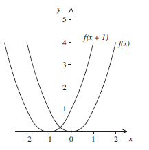
The graph of y = f(x) is mapped onto f(x + 1) by a translation of 1 unit to the left.
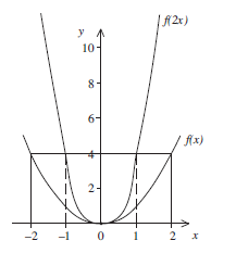
The curve for f(2x) is much steeper than for f(x). This is because the curve has been compressed by a factor of 2 in the x-direction. Compare the rectangles ABCD and EFGH.
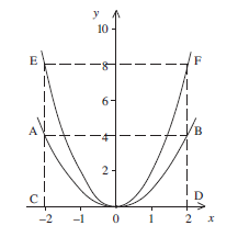
Here the curve y = f(x) has been stretched by a factor of 2 in the vertical or y-direction to obtain the curve y = 2f(x). Compare the rectangles ABCD and CDFE.
Note that if k is negative and k < −1the curve will be stretched and reflected in the x-axis while if −1 < k < 1, it is compressed.
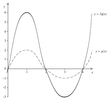
The graph below shows y = g(x) .

On separate diagrams show:
y = g(x) and y = g(x − 1)
To obtain y = g(x − 1) translate y = g(x) 1 unit to the right.

y = g(x) and y = g(2x)
To obtain y = g(2x) compress y = g(x) by a factor of 2 horizontally.

y = g(x) and y = 3g(x)
To obtain the graph of y = 3g(x) stretch the graph by a factor of 3 vertically.
Exercises
